Those working with sediment cores often use sample depth as a proxy for sample age. If radiocarbon dates are available, it is useful to convert depth units into equivalent C-14 years. When I ask my students to do this as an exercise, I have always been fascinated with their attitudes; most will accept without question a carbon date and its stated error. When deeper dates show constant age, or when younger dates lie under older ones, students put absolute trust in nuclear physics and readily discard pollen zone boundaries, principles of superposition, and Ockham's razor. Sediment processes in lakes can be complicated, of course, but there are many reasons why carbon dates can be in wrong as well.
A student will often construct a depth-age plot, connect the dates with straight line segments, and use some kind of linear regression to assign ages to the depth samples. This involves a lot of work; it is no small task to convert a pollen diagram from depth to age--let along considering different kinds of regression. Tedious tasks keep us from looking at interesting questions. For one thing, the slope of a line connecting two dates is a measure of the net rate of sedimentation (cm/yr) between the dated points. I recall a student's comment when he noted his sedimentation rates were always constant in the interval from one date to the next, but would then change and become constant again on the way to the next date in sequence. He thought it was neat how the carbon dates had been able to "catch" these rate changes!
Partly as a result of that experience, I developed a PC-based program which allows one to make a depth-age plot on a graphics screen. Age can then be regressed on to depth by fitting exponential, power, or nth-order functions, as well as doing linear and cubic splines regressions. Using this program, a student can quickly learn that the same data can be fitted by different functions, and those that are best in one situation may do poorly in another. A function's parameters can be saved in a "rate" file. A rate file can be used to take one of my POLFILE data files ordered by depth and automatically convert it to a file ordered by age. The implied sedimentation rate at each sample level is calculated as well.
I call this program DEP-AGE; it functions by reading depth and age data from an ASCII file with the three-letter extension "C14" after its name. I will use a restricted data set from my Devils Lake core as an example of the operation. DEV9WTOP.C14 (short for Devils Lake; 9 samples with the top 0.5 cm assigned the date the core was taken: 1978 AD = -28 BP.) is shown below:
Devils Lake, Sauk Co., WI
 4
 9
MinDepth(cm)
 0 164 263 334 395 455 514 541 599
MaxDepth(cm)
 .5 169 267 338 399 459 518 547 611
C14Age(YrBP)
 -28 2430 4105 5245 6920 8640 10080 10620 12550
StandDevAge
50 65 65 65 75 85 100 105 132
It consists of a title line, followed by the number of categories (4), and the number of dated points (9). The program assumes all depths will be in centimeters and all ages in years. Each dated interval has a top (MinDepth) and a bottom (MaxDepth) and an age with a standard deviation. In the *.C14 file above, the first actual carbon date came from the interval from 164 to 169 cm in the core; its reported value was 2430 ± 65 BP.
This kind of file can be made with an ordinary word processor or with POLFILE. If you use POLFILE, first make a RAW file of the four categories: MinDepth, MaxDepth, Age, and StandDevAge. Then make it into a DATA file called ANYNAME.C14.
Starting Dep-Age, produces the following menu:
1. Plot Diagram Regressing Age (Years)
      on to Depth (Centimeters). The program
      gets data from a '*.C14' file.
2. Information About Making a '*.C14' File.
3. Calculate Age of Sediment Level, Given Depth.
Q. Quit!   ( Use this to END the Program. )
                     Choose 1, 2, 3, or Q _
If you select "1" and load DEV9WTOP.C14, the screen will plot the depth-age
chart with the nine control points shown in fig. 1.
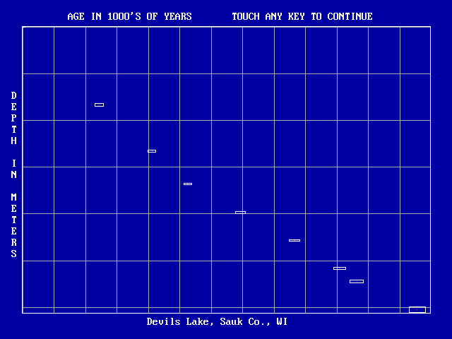
 Results of DEP-AGE.EXE
Devils Lake, Sauk Co., WI

N-categories = 4   N-samples = 9

CATEGORIES IN FILE: DEV9WTOP.C14
MinDepth(cm)  MaxDepth(cm)
       C14Age(YrBP)  StandDevAge

1. SHOW Diagram of Site.
2.   TOGGLE Graph ORIGIN Top to Bottom.
3. FIT Nth ORDER CURVE to Control Points.
4. FIT EXPONENTIAL CURVE to Control Points.
5. FIT POWER CURVE to Control Points.
6. FIT CUBIC SPLINE to Control Points.
7. INTERPOLATE LINEARLY between Control Points.
8. **SAVE CURVE DATA TO A DISK FILE**
9.   CHANGE Site.
C.         Change COLORS of Screen.
Q.         QUIT and Return to First Menu.
                     Press 1 - 9 , C, or Q _
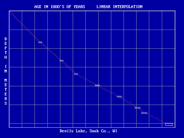
Picking "7" produces the chart shown in fig. 2. Because these lines are one
measure of sedimentation rate (cm/yr) in the core, it may help if rates are
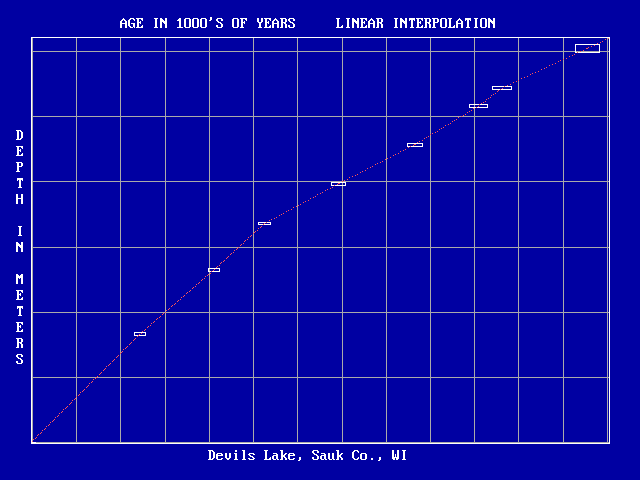
drawn with positive slopes. In that case touch "2", and the graph is redrawn
so that both depth and time increase up and right (fig. 3). (My student
would note that the carbon dates had again miraculously captured the places
where the sedimentation rates changed.) Touch any key again to return to the
menu.
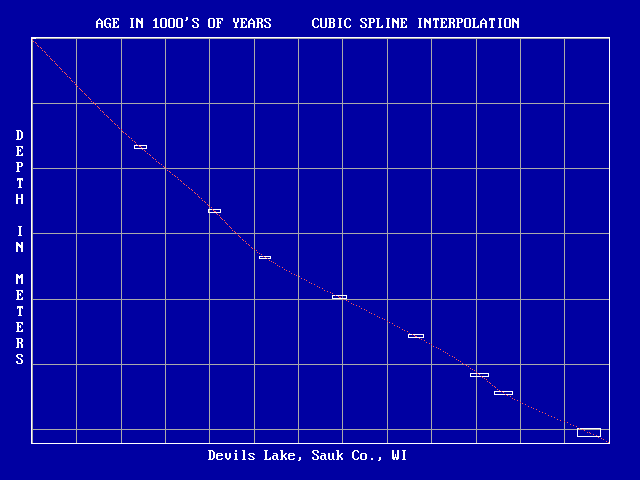
Touching "4" or "5" will fit, respectively, exponential or power functions to the data. These functions were commonly used before computers; exponential functions plot as straight lines on semi-log paper, and power functions plot as straight lines on log-log paper. Exponential rates are common in Nature, but relatively rare in sedimentation. Power functions often do a reasonable job in describing sedimentation. Both are "unidirectional," and this agrees with our prejudice that as sediments go deeper, they should get older.
I like to pick "3" and fit an nth-order function to the control points. Recall that a first-order function is a straight line, a 2nd-order function is either convex or concave, but does not change between the two. In general, nth-order polynomials have n-1 bends, and this helps us predict what order will be required to match the data. Assume that you pressed "3." You will be asked what degree of equation is to be fitted (i.e. 1, 2, 3 ...). If you select 2, the following will appear on the screen:
  [ control points not shown here ]
               Constant = 2.612551
 1   Degree coefficient = 11.15511
 2   Degree coefficient = 1.585796E-02
Coefficient of determination
                 (R-squared) = .9986199
Coefficient of determination = .9993097
  Standard error of estimate = 177.6288
Perhaps you have shared with me the humiliation of hearing a colleague talk
about fitting a 5th-order function to his/her dates, when you could not do
the math. Without a computer and the right program, one
is restricted to sketching on log paper or fitting curves by "eye-ball."
DEP-AGE lets you do reconnaissance curve-fitting in the privacy of your PC.
Fitting a mathematical curve to the data by regression does not imply that
the lake "has a memory" such that its early sedimentation rate predicts later
values. Rather, we try to choose a reasonable function and then fit it so
that its deviation from all the control points is minimized. A 5th-order
curve does a good job of running a smooth line near most of the dates in the
DEV9WTOP.C14 file. But a 2nd-order polynomial does almost as well (fig. 5).
I tend to experiment by fitting a variety of curves, then taking the lowest
order than does a reasonable job. The curve in fig. 5 passes through the
error boxes of eight of the nine control points, and it grazes the ninth.
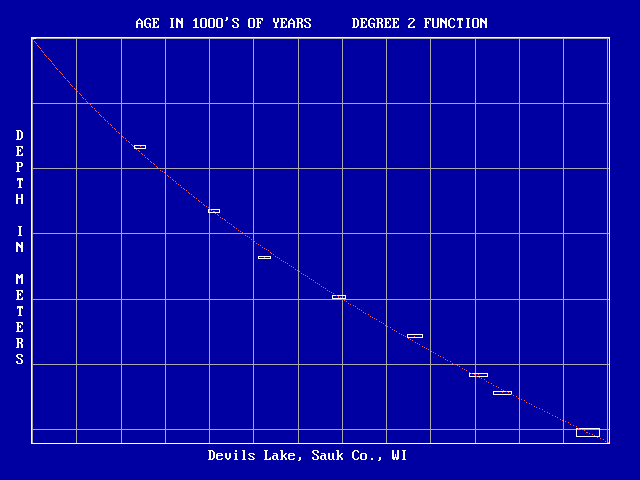
Devils Lake, Sauk Co., WI    01-05-1992
Control Points = 9  Polynomial of degree 2
             Constant = 2.612551
 1 Degree coefficient = 11.15511
 2 Degree coefficient = 1.585796E-02
Coefficient of determination
                 (R-squared) = .9986199
Coefficient of determination = .9993097
  Standard error of estimate = 177.6288
      Control Points
Sample DEPTH   Sample AGE
       0.3          -28
     166.5         2430
     265.0         4105
     336.0         5245
     397.0         6920
     457.0         8640
     516.0        10080
     544.0        10620
     605.0        12550
The *.RAT file varies somewhat for each different function fit to the data,
but is basically self-explanatory. It is an ASCII text file that can be
examined easily. However, avoid editing a *.RAT file because DEP-AGE uses
the format to recognize the function and read the parameters. After saving
a *.RAT file, press "Q" to return to the first menu. When you then select
"3. Calculate Age of Sediment Level, Given Depth," you will be asked for the
name of the desired *.RAT file. Assuming it is DV-2ND.RAT, when the file is
read, the computer screen will show the function's parameters at the top,
whereas instructions and the depth of lowest control point are at the bottom.
(Remember: only a fool extrapolates a polynomial curve outside the range of
its control points.)
Devils Lake, Sauk Co., WI    01-05-1992
Control Points = 9  Fit to Polynomial of degree 2
             Constant = 2.612551
 1 Degree coefficient = 11.15511
 2 Degree coefficient = 1.585796E-02
                           (R-squared) = .9986199

 Depth(cm) = 600   Age = 12405   Cm/Yr = 0.0331
 Depth(cm) = 500   Age =  9545   Cm/Yr = 0.0370
 Depth(cm) = 400   Age =  7002   Cm/Yr = 0.0419
 Depth(cm) = 300   Age =  4776   Cm/Yr = 0.0484
 Depth(cm) =
        ----------------------
ENTER DEPTH IN CENTIMETERS TO ESTIMATE C14 AGE
       [ CR ALONE TO EXIT ]
  Lowest control point is 605 centimeters.
        ----------------------
When the depth value is typed, the predicted age is supplied along with an
estimate of the sedimentation rate at that depth. The sedimentation rate
(cm/yr) is taken as the reciprocal of the difference in estimated age at the
top and base of the 1-cm interval centered on the specified depth. I use
this method rather than reporting rate as the tangent to the curve at the
specified depth; most sediment samples are not dimensionless "point" samples.
This screen allows one to try a few values to test the general results of the function. Pressing "enter" or "carriage return" without specifying a depth, gets you back to the initial menu, but you are first given the opportunity of converting one of POLFILE's data files ordered by depth to a *.DAT file ordered by age in years. (An alternate choice is age in decades; see below.)
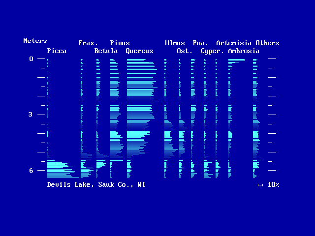
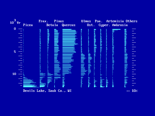
My *.DAT files have a title, an integer representing NP, the number of pollen taxa, and an integer representing NS, the number of samples. Given this information, an array of pollen data can be read for computer processing; the actual distance (depth) between the samples is often not needed. But I include ordinal data at the end of the pollen data. If such data are required, the program expects to find this information after the pollen data; it merely reads in NS values of depth. But there is no reason why these NS values must be depth; they might well be years or decades. My program PLOTSITE reads a *.DAT file, and it normally reads the extra ordinal sample depths (cm) to use in plotting a simple pollen diagram. PLOTSITE defines the y-axis by plotting a short marker at 100-cm intervals. Now if the ordinal depth units were replaced with age in decades, PLOTSITE's y-axis indicators will mark off 100 decades or 1000 years. Figure 6 represents a restricted data set from Devils Lake whose core is a little over 6 meters long. Figure 7 shows the same data, but with the y-axis scaled in 1000's of years based on the 2nd order fit of DV-2ND.RAT.
Devils Lake, Sauk Co., WI
 12
 31
Picea
 1 0 0 0 1 1 1 0 0 1
 0 0 1 1 0 0 1 1 1 0
 1 0 2 23 30 129 188 127 196 264
 225

...[10 taxa deleted]...

Other Terrestrial Types
 78 70 68 50 80 69 54 55 53 70
 56 75 62 49 58 87 117 86 79 89
 176 103 106 213 110 220 163 311 149 142
 98
Depth (cm)
 .5 19.5 46.5 76.5 104.5 130.5 154 174 194 214
 234 259 278 298 318 344 364 384 404 430
 449 469 489 509 535 554 570 584 598 608
 628
'Subset of Devils Lake core for Newsletter'
The derived *.dat file ordered by age contains additional information:
 ....

Other Terrestrial Types
 78 70 68 50 80 69 54 55 53 70
 56 75 62 49 58 87 117 86 79 89
 176 103 106 213 110 220 163 311 149 142
 98
Estimated Age in Decades BP
 1 23 56 95 134 173 210 242 276 312
 348 396 433 474 515 572 616 662 710 773
 821 872 925 979 1051 1105 1151 1193 1234 1265
 1326
Estimated Sedimentation rate in cm/yr
 .089 .085 .079 .074 .069 .065 .062 .06 .058 .056
 .054 .052 .05 .049 .047 .045 .044 .043 .042 .040
 .039 .038 .038 .037 .036 .035 .034 .034 .033 .033
 .032
Depth (centimeters)
 .5 19.5 46.5 76.5 104.5 130.5 154 174 194 214
 234 259 278 298 318 344 364 384 404 430
 449 469 489 509 535 554 570 584 598 608
 628
'Subset of Devils Lake core for Newsletter'
Age in Decades were converted from original
Depth(cm) by the following:
Devils Lake, Sauk Co., WI    01-05-1992
Control Points = 9  Polynomial of degree 2
             Constant = 2.612551
 1 Degree coefficient = 11.15511
 2 Degree coefficient = 1.585796E-02
Coefficient of determination
                 (R-squared) = .9986199
Coefficient of determination = .9993097
  Standard error of estimate = 177.6288
      Control Points
Sample DEPTH   Sample AGE
       0.3          -28
     166.5         2430
     265.0         4105
     336.0         5245
     397.0         6920
     457.0         8640
     516.0        10080
     544.0        10620
     605.0        12550
The sample ages and sedimentation data are added after the pollen data, and
the original depths and the *.RAT file are appended for purposes of
documentation. A word processor can be used to cut/copy the derived ages and
sedimentation rates from the file to be pasted into a file for use with Craig
Chumbley's PALYPLOT. Or the *.DAT file can be edited with POLFILE to Eric
Grimm's "Wisconsin" format for importation into TILIA. I would be happy to
provide a free copy of DEP-AGE, POLFILE, and PLOTSITE, if you provide me with
a blank formatted disk, tell me what kind of graphic screen you use (EGA,
VGA, or MCGA), and whether you have a color or black and white monitor.
References
Chumbley, C. A. 1991. PALYPLOT: A PC-based program for plotting pollen and plant macrofossil stratigraphic data. INQUA - Commission for the Study of the Holocene, Working Group on Data-Handling Methods Newsletter 5: 2-4.
Grimm, E. C. 1990. TILIA and TILIA·GRAPH: PC spreadsheet and graphics software for pollen data. INQUA - Commission for the Study of the Holocene, Working Group on Data-Handling Methods Newsletter 4: 5-7.
Maher, L. J., Jr. 1990. Programs useful in the pollen lab. INQUA - Commission for the Study of the Holocene, Working Group on Data-Handling Methods Newsletter 4: 7-10.