MODPOL.EXE: A TOOL FOR SEARCHING FOR MODERN ANALOGS OF PLEISTOCENE POLLEN DATA
Louis J. Maher, Jr.
Department of Geology and Geophysics
University of Wisconsin
Madison, WI 53706
USA
Geologists state that the present is the key to the past. Quaternary pollen diagrams are often indirectly interpreted by comparing their pollen spectra with modern sites that have similar pollen proportions. But until now the average student pollen analyst has faced a difficult task in trying to compare fossil and modern sites. MODPOL.EXE is a program designed to allow the easy comparison of levels in a fossil pollen diagram with modern surface samples from the non-mountainous regions of North America. The modern pollen data are an edited subset of the M70 modern pollen sequences available from the National Geophysical Data Center at:
ftp://ftp.ngdc.noaa.gov/paleo/pollen/asciifiles/modern/napd/
Let me make a generalization at this point, and I will try to defend it during the remainder of this article. Information from modern pollen studies can be very interesting and potentially very valuable; it can also be difficult to evaluate and at times be very frustrating.
In this discussion of MODPOL (MODern POLlen) I am going to use the North American Pollen Database's Weber Lake diagram that was fashioned by concatenating two of the pollen diagrams that were published by the late Magnus Fries (1962). I have fond memories of Magnus as a kind and patient gentlemen who helped initiate my pollen career by drawing clear sketches of the common pollen grains and surviving a deluge of naive questions while he was a visiting researcher at the University of Minnesota.
For the smoothest action you should run MODPOL.EXE using the full screen. If you find yourself in a small window, click on the "full-screen" icon at the top of the window. You can later restore your small DOS screen by right-clicking the DOS icon on your desktop, pick properties/screen and click "window".
At MODPOL's initial screen, touching "1" automatically loads "PLOT.INF" (a file containing screen-plotting information) and "Mod1," the first of 15 modules of modern pollen data; altogether these modules contain information from 1924 sites. You will then see a listing of all of the fossil pollen data files (*.dat) in the default directory. You can make your own fossil pollen data files later. Until you do, Weber Lake and other example files are available with which you can experiment. Touching "2" displays help material based on the text you are now reading.
When you type in the complete name of the fossil site from the list on the screen--in our example: WEBER55.DAT--the program loads that file and immediately calculates the fossil and modern proportions and squared-chord dissimilarity coefficients (DC) between each level in Weber Lake with each level in Mod1. If you are using a fast Pentium-type computer, the computation will take about three seconds; if you are using an old 286-type machine, it may take three minutes. You will be asked for a short name for your fossil site for use on the screen. When the calculations are finished, you will see an initial screen that lists the names of the two sets of data, a summary of their size, a list of the 55 taxa that are contained in the data, and a menu of possible choices of action.
1. ** EXAMINE DC MATRIX **
2. Load New Section of Modern Pollen Database
3. Load New Fossil Pollen Diagram
4. Help
5. EXIT ( Use this as your last choice ! )
Normally at the start you would choose item 1. The first time you make this choice you will encounter a screen that describes the color scale used for the dissimilarity coefficients. The squared-chord DC can range from 0 (the two samples are exactly alike) to 2 (the two samples have no taxa in common). You are offered a default value of 0.2 as the maximum DC to display. Overpeck et al. (1985) used 0.15 as their "critical" value in deciding analog/no-analog conditions. For reasons I will touch on, I am suggesting that we use 0.2. You can accept the default by pressing the <enter> key, or you can type in another number. MODPOL does not display DC values greater than 0.7; as you will discover, sites yielding DCs at that level are quite different.
Figure 1, shows the DC matrix screen. The matrix may contain many small colored squares or it may show nothing but a blank grid. In the case of Figure 1 we see only six tiny red squares. First examine the margins of the central rectangle. You will see the names of the X- and Y-axes at the top of the screen. The parentheses (YUK and NWT) along the top margin contain abbreviations of the Canadian Provinces (three letters) or the US States (two letters) that appear in the modern pollen module being displayed. In this case the sites are from the Yukon and the Northwest Territories. The word "TOP" at the upper left margin indicates the top of the fossil core. At the upper part of the right margin you see a key to the colors that may appear on the matrix. Under the color key you will see the line "DC = SqCHD" which reminds you that the dissimilarity coefficients are based on the squared-chord criterion. You will also see the value of the maximum DC that is currently displayed; if you accepted the default, it will indicate .200.
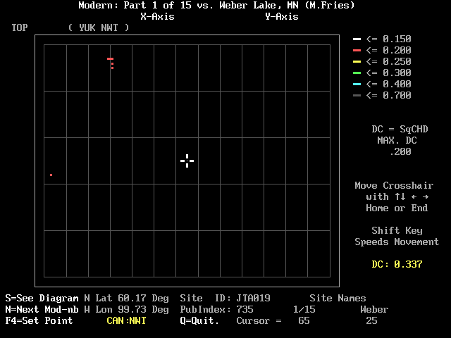
Next below are some instructions for moving the cursor, the white cross that appears near the center of the array. You move the cursor with the <arrow> keys; holding down the <shift> key will generally move the cursor faster. The <home> key will move the cursor to the top left of the array; the <end> key will move it to the lower right. Just below the cursor instructions you will see in yellow the value of the DC where the cursor is presently located; in this case 0.337. This is one of the numbers in the margin that will change as the cursor moves.
The short site names are shown at the right side of the lower margin. When you start, the modern pollen module will be called "1/15"; this will change later to "2/15", "3/15 ", ..."15/15." The numbers under these short names refer to the cursor coordinates. Moving the cursor up or down changes the level number of the fossil site; moving the cursor left or right changes the modern site. You will notice that a number of changes occur in the margins when the cursor is moved left or right. The latitude and longitude will change to indicate the geographic position of the modern site; its Province or State will be shown in yellow. Site ID indicates the modern site's identity name in the M70 database. The Publication Index (PubIndex) will show a number. The Site ID and the PubIndex will allow you to look up what is published about that site in "REF-CIT.TXT," an ASCII file of reference citations that can be found in the MODPOL directory. A PubIndex number of 0 indicates that the modern sample was not actually published by the palynologist who counted the sample; the SiteID of such a site often contains letters that look very much like the collector's initials. For example, the cursor in Figure 1 rests on site JTA019, the 65th site in the module " Modern: Part 1 of 15" that has a Publication Index of 735 which corresponds to Andrews and Nichols (1981), a site in the Northwest Territories at 60.17 degrees N, 99.73 degrees W. The DC between this site and level 25 in Weber Lake is 0.337; it is blank on the array because it is greater than the maximum DC (0.200) we chose to show by color.

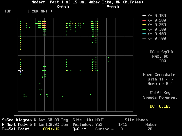
In Figure 2 the cursor has been moved to the red square at the 3rd site in the module: HAIL (Cwynar, 1995) in the Yukon. The DC between it and Weber Lake level 28 is 0.163. Besides the <arrow> keys that are used to move the cursor, you can type numbers, and certain other keys have special functions. To change the maximum DC that is displayed in color, simply type a decimal point (.) followed by a number (i.e. .312; 0.312 will also work); then touch the <enter> key. (If you should type other punctuation [comma, most letters, etc.] the program will interpret the input as a zero, and no color codes will appear; to recover, simply type a new number. As mentioned earlier, any number greater than .7 will default to 0.7.) Figure 3 is similar to Figures 1 and 2 except that I typed 0.3. There are now many points of yellow and green.
Four keys having special functions are shown in bright white in the lower margin. These are "S", "N", "F4", and "Q". Figure 4 shows what happens when you touch "S" when looking at the screen shown just above. "S" lets you see a schematic pollen diagram of the fossil site and the modern site that correspond to the position of the cursor. The modern site's diagram in bright yellow appears just below the taxon names. The fossil site's diagram appears below with the level equivalent to the cursor in bright yellow. The two diagrams are separated by a scale showing the length equivalent to 20 per cent of the pollen sum.
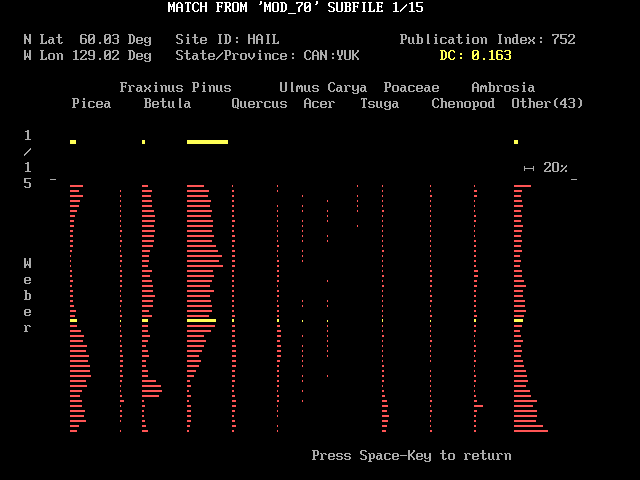
Information about the modern site is displayed at the top of the screen, and the dissimilarity coefficient at the cursor is shown in yellow. Although a DC of 0.163 seems quite good, notice that while twelve taxon columns of Weber lake are occupied, only 4 columns are lit in HAIL. That kind of observation is probably worth pondering when deciding whether one has found a modern analog. Touching the <space> key returns you to the screen with the DC array; any other key elicits a "blip" sound. Normally you will first pick a position of a white (DC <= 0.15) or red (DC <= 0.2) square on the DC array before touching "S" to see how the sites match. But when you are first starting with MODPOL you may want to put the cursor on an unlighted square with a large DC value; touching "S" can then show you how poor matches look, and this helps give meaning to the dissimilarity coefficients.
Touching "N" from the DC array screen loads the next modern pollen module and calculates the new DC matrix. You can continue loading in new modules by pressing "N" until you reach a screen with more reds and whites that suggest good matches. When you finish with modern pollen module Mod15, pressing "N" again reloads Mod1. You will learn below how to load a specific modern pollen module of your choice.
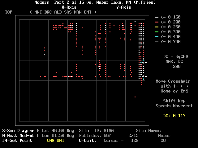
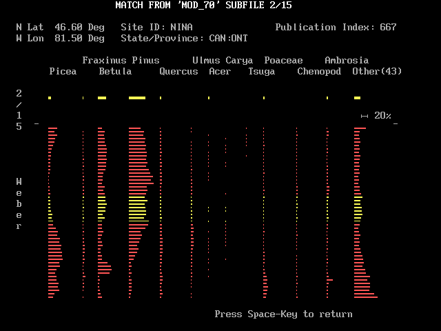
The DC array screen may at times exhibit a short column of "hot" white or red colors that indicate an interval or "zone" in the fossil data that match a particular modern site. Figure 5 shows an example near the right margin at the NINA site (Liu, 1990) in Ontario. If you place the cursor on one end member of the low-DC column and press the <F4> key you will hear a low beep. If you then move vertically to the other end of the bright column and press the <F4> key again, you will switch to the pollen diagram screen shown in Figure 6. The part of the fossil diagram that corresponds to the bright column will be high-lighted in yellow. The screen is nearly the same as the one previously reached by typing "S". However in this case no discrete DC value is shown; the DCs vary within the range of their color code in the array. As instructed at the base of the pollen diagram, touch the <space> key to return to the DC array.
The last of the four control keys shown on the DC array screen is "Q" to quit the screen. (The <Esc> key will also produce the same result.) On pressing <Q> or <Esc> you will be back at the menu screen with the following choices:
1. ** EXAMINE DC MATRIX **
2. Load New Section of Modern Pollen Database
3. Load New Fossil Pollen Diagram
4. Help
5. EXIT ( Use this as your last choice ! )
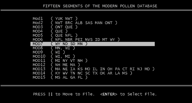
If you press "2" you will see a screen with a list of the 15 modern pollen modules that is similar to Figure 7. You can use the up or down arrows to move the bright bar to the module of your choice. You will note that the geographic locations of the modern sites in each module are indicated by the Province and State abbreviations at the right of each module name. When the desired module is highlighted (MOD7 in this case), pressing the <enter> key will load the module and calculate the DCs. You will be returned to the menu where you can examine the DC array by pressing "1".
By pressing "3" you can load a new fossil diagram and recalculate the DC matrix. Pressing "4" gets you to the Help sequence. Press "5" to exit from the program.
ADAPTING A FOSSIL POLLEN DIAGRAM FOR USE WITH MODPOL
To adapt your own pollen diagrams to use with ModPol, you must assemble your data so that they match the sequence in the example files. The ASCII file TAX55.TAX provides the names of the taxa in correct sequential order. You may have to group some of your taxa (combining multiple pine types into the single taxon Pinus, multiple walnuts into Juglans, etc.). This can be done using Eric Grimm's Tilia or Tilia2 (Grimm, 1991). When you are satisfied, from the Tilia menu screen, select "D. Save data file," and then "F. Wisconsin format." The saved data file should have the extension ".RAW". This raw file can be read into POLFILE.EXE, a program you will find in your MODPOL directory. When you run POLFILE.EXE you will see the following menu:
1. Make a RAW FILE
2. Make a DATA FILE from a RAW FILE
3. -Consolidate Columns in a Raw file
4. -Change Taxon Order in a Raw file
...
9. ------Discussion and help
Choose "9" to review POLFILE options. Selecting "3" allows you to combine taxa (i.e. pines) which are then stored at the end of the file (TotalPine, TotalJuglans, etc.). If you wish to change the order of the taxa, select "4". When you are satisfied, choose "2" to make a *.DAT file from the *.RAW file. When you are asked how many taxa will be in your new file, type in 55. When you are asked for the order of the taxa in the *.DAT file, type the name TAX55.TAX which will be loaded to use as the source that will allow your *.DAT file to match the modern pollen modules. If the required taxon is not found in your data, choose "0. NOT INCLUDED." The fossil data file must have the extension ".DAT" whether it is added automatically or typed by you. When you are asked what value to use to order the sample levels, choose zero (0) , Level Number. This will order the fossil levels in the sequence 1, 2, 3,...n which is required for MODPOL. (This option was first available in POLFILE.EXE version 1.17.)
You will also find MAKE_INF.EXE in your MODPOL directory. MAKE_INF can be used to edit the file PLOT.INF (plotting information) that controls the taxa (and their spacing) shown in MODPOL's pollen diagrams. A back-up copy of PLOT.INF is contained in the file PLOT-HLD.INF. If you are not satisfied with your edited PLOT.INF, from DOS, type
COPY PLOT-HLD.INF PLOT.INF
and you will be back where you started.
MODPOLZ.EXE, a self-unzipping file, can be obtained at the INQUA File Boutique at www.chrono.qub.ac.uk/inqua/boutique.htm or at the mirror site at www.geology.wisc.edu/~maher/inqua.html.
Make a "MODPOL" directory, put MODPOLZ.EXE in it, and type its name to expand all the files you need to get started using it.
PROBLEMS INVOLVED IN SEARCHING FOR MODERN ANALOGS OF FOSSIL DATA
It is very satisfying to find modern pollen sites that closely match portions of our fossil cores. One feels that the climatic parameters of the modern site must tell us something of the conditions our site experienced. But there are a number of reasons why we should temper our enthusiasm with a certain amount of scepticism.
For one thing the modern data were contributed by many individuals with differing interest in the intricacies of pollen taxonomy. I will admit, however, that MODPOL shows me there is an impressive degree of consistency in the counts in the various geographic regions. The modern samples come from different depositional environments--lake mud, peat, surface soil, moss, etc.--and each environment favors certain taxa over others. While the M70 database does contain information about some of the samples, the terms may be vague or absent.
One problem especially noticeable in the central part of the U.S. is that the modern samples were taken after a century and a half of intensive agriculture which produced the well-known "Ragweed Rise." The file DEV55.DAT from my site at Devils Lake, WI. is included in the MODPOL directory. If it is compared with the surface data site DEVILSWI (Mod8, number 77) only 16 levels have DC values less than 0.2. The top level of the core has a DC of 0.000 which is satisfying, but the modern sample does not truly represent the pollen deposition at the time before European settlement. There have been a few studies (i.e. McAndrews, 1966, Plate 2) where workers have selected samples from just below the Ambrosia rise to avoid this problem, but that requires orders of magnitude more work. One could try to mitigate the problem by deleting Ambrosia-type from the pollen sum; however that would prevent the ragweeds from being used to document disturbance or dry times in the earlier record.
Another problem arising from comparing fossil and modern samples--or comparing any pollen samples for that matter--is that no two analysts could ever recount their samples and arrive at exactly the same numbers; yet the dissimilarity coefficients are based only on the initial counts. Therefore one must view the DC as an approximation. In the initial count the two samples may meet some assumed "critical " value and be judged to meet the criterion as a modern analog. If one or both of the samples were recounted, the calculated DC might fail the test. Another problem with DCs that is not so obvious is that the calculated value is not independent of the number of taxa in the counts. MODPOL uses 55 taxa in its calculations. If 25 taxa had been used, the value of the mean DC in the arrays would be a few percent less than the mean when 55 taxa are used.
Difficulties in the hunt for modern analogs have been discussed a great deal. Figure 8 illustrates a very common situation. Here we are looking at Weber Lake and Mod7. The maximum color-coded DC that MODPOL will show is 0.7. Sites with white and red DC are pretty much restricted to Weber Lake levels above 35. This pattern is repeated in the next three modern pollen modules. Notice how many of the DCs are 0.7 or larger. Level 35 in Weber Lake corresponds to a depth of 620 cm with radiocarbon age of about 9500 yr B.P. (The fossil-pollen files supplied with MODPOL have such information attached at the end; you can read it in a separate DOS window with a simple text reader like "EDIT" that comes with Windows .)
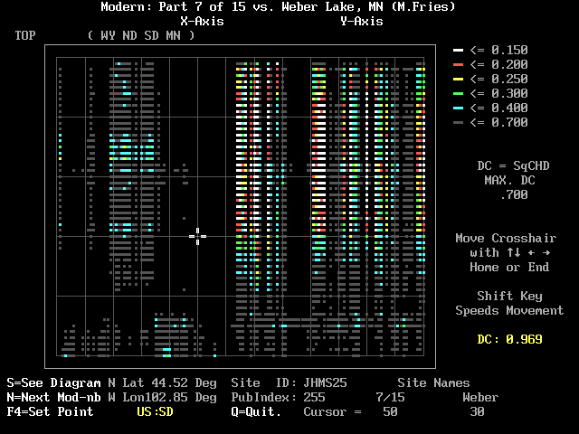
What this demonstrates, of course, is that the early part of the interval--as short even as the Holocene--has pollen assemblages that cannot be matched with modern samples in the extensive M70 dataset. That this was caused by postglacial vegetation migration was well shown by Bernabo and Webb (1977). Wright (1968) called our attention to the fact that Late-Glacial forests in the Upper Midwest lacked pine. Although pollen analysis has established that pine was abundantly mixed with spruce in the north-central U.S. during earlier interstadials, it had become locally extinct before the last ice sheet retreated. Since then many workers have traced the separate movements of red pine--and later white pine--into the area. Late-comers like beech and hemlock arrived west of Lake Michigan only within the last half of the Holocene. Today's Boreal forest in central Canada has a good deal of pine mixed with the spruce; modern pollen samples from that area cannot be expected to match the pine-poor spectra of the Late Glacial. Is the present the key to the past? If individual members of the flora migrate at different rates and routes, can there really be modern analogs of past vegetation? I suggest you work with MODPOL for an evening and draw your own conclusions. It will be an interesting enterprise and your students may enjoy it as well. Besides Weber Lake, I have included several other pollen diagrams for you to try before you adapt those of direct interest to you. These include: Eagle Lake Bog (Spear, 1981), Devils Lake (Maher, 1982), Kirchner Marsh (Wright, Winter and Patten, 1963), Pickerel Lake (Watts and Bright, 1968 ), and Volo Bog (King, 1981). Please look at the file REF-CIT.TXT to gain an appreciation of all those who contributed their work to the M70 database.
DATA SELECTION FROM THE M70 DATASET
The M70 Dataset includes material from 59 US States and Canadian Provinces. For this project I wished to emphasize the Eastern Lowlands of North America. Therefore I omitted data from the following eight states: Alaska, Arizona, California, Colorado, New Mexico, Oregon, Utah, and Washington.
The 51 states and provinces that I used contained data for 71 taxa from 2365 sites. I felt it necessary to do some preliminary filtering of the data which had the effect of reducing the number both of the taxa and the sites. As an example, in the original data three categories of Pinus were recorded: Pinus subg. Pinus, Pinus subg. Strobus, and Pinus undiff. While it is good to keep subgroups separate in databases, it can confuse the issue for my purposes when numerous authors contribute information; some routinely attempt to divide the pine genus--others simply record pine. If two such analysts were to study adjacent sites, one would have information in all three pine categories, the other would have data only for Pinus undiff. The squared-chord DC values might appear quite different merely because of their definition of pine. For the same reason I consolidated four Tsuga categories into one.
I discarded the two categories "other trees and shrubs" and "other herbs" because they lacked any real meaning; two sites might have similar numbers of grains in these categories, but include none of the same taxa. I grouped Iva with Ambrosia as Ambrosia-type because some analysts group all short-spine Compositae as Ambrosia-type. Cerealia was grouped with Poaceae. Cercocarpus-type--two grains reported in only one sample--was added to Rosaceae. Ericaceae and Ericales undiff. were combined as Ericales. Rumex and "Rumex/Oxyria digyna undiff" were combined as Rumex-type. The categories Ceanothus and Eriogonum were deleted; they each occurred as a single grain in only one sample. Lastly the category Euphorbia-type was deleted as it never did occur in the 51 state/provinces I had selected for this study. With this editing, I ended up with the 55 taxon categories that are found in the ASCII file TAXA55.TAX.
Whether the number of taxa is 71 or 55, one would hope the counts contain a sufficient number of grains to yield reasonable estimates of each taxon's abundance. (Twenty-two of the samples had 50 or fewer grains; five had less than 11 grains.) I arbitrarily decided to restrict this study to samples with at least 200-grains sums. This reduced the number of sites from 2365 to 1924. (Because I later discarded the categories "other trees and shrubs" and "other herbs" 15 of the final 1924 sites contained fewer than 200 grains; nonetheless they were retained.)
The 1924 modern surface samples in the 15 modules could be arranged in any order, say by either latitude or longitude. I simply used the geographical position of the Canadian Provinces and US States running in west to east swaths starting at the north and ending at the south.
References:
Andrews, J.T. and Nichols, H. 1981. Modern pollen deposition and Holocene palaeotemperature reconstructions, central northern Canada. Arctic and Alpine Research 13(4):387-408.
Bernabo, J.C. and Webb, T. III. 1977. Changing patterns in the Holocene pollen record of northeastern North America: A mapped summary. Quaternary Research 8:64-96.
Cwynar, L.C. 1995. Paleovegetation and paleoclimatic changes in the Yukon at 6 ka BP. Géographie physique et Quaternaire 49:29-35.
Fries, Magnus. 1962. Pollen profiles of Late Pleistocene and Recent sediments from Weber Lake, Minnesota. Ecology 43:295-308.
Grimm, E. C. 1990. Tilia and Tiliagraph: PC spreadsheet and graphics software for pollen data. INQUA-Commission for the Study of the Holocene, Working Group on Data-Handling Methods Newsletter 4:5-7.
King, J. E. 1981. Late Quaternary vegetational history of Illinois. Ecological Monographs 51(1):43-62
Liu, K.-B. 1990. Holocene paleoecology of the boreal forest and Great Lakes-St. Lawrence forest in northern Ontario. Ecological Monographs 60:179-212.
Maher, L.J., Jr. 1982. The palynology of Devils Lake, Sauk County, Wisconsin. Pages 119-135 in J.C. Knox, L. Clayton, and D.M. Mickelson, editors. Quaternary History of the Driftless Area: Wisconsin Geological and Natural History Survey Field Trip Guide Book Number 5, University of Wisconsin-Extension, Geological and Natural History Survey.
McAndrews, J. F. 1966. Postglacial history of prairie, savanna, and forest in northwestern Minnesota. Memoirs of the Torrey Botanical Club 22(2):1-72, 6 plates.
Overpeck, J. T., Webb, T., III, and Prentice, I. C. (1985). Quantitative interpretation of fossil pollen spectra: Dissimilarity coefficients and the method of modern analogs. Quaternary Research 23:87-108.
Spear, R.W. 1981. The history of high-elevation vegetation in the White Mountains of New Hampshire. Dissertation. University of Minnesota, Minneapolis, Minnesota, USA.
Watts, W.A., and Bright, R.C. 1968. Pollen, seed, and mollusk analysis of a sediment core from Pickerel Lake, northeastern South Dakota. Geological Society of America Bulletin 79:855-876.
Wright, H. E., Jr. 1968. The roles of pine and spruce in the forest history of Minnesota and adjacent areas. Ecology 49(5): 937-955.
Wright, H. E., Jr., Winter, T. C., and Patten, H. L. 1963. Two pollen diagrams from southeastern Minnesota: problems in the regional Late-Glacial and Postglacial vegetational history. Geol. Soc. of America Bull. 74:1371-1396.